¶ Understanding the Poisson Distribution
The Poisson distribution is a discrete probability framework used to model the frequency of independent events occurring within a fixed interval of time or space. It relies on a foundational constant, denoted by the Greek letter lambda (), which represents the average rate of occurrence. For the distribution to hold true, events must happen independently, at a constant average rate, and cannot occur simultaneously.
¶ Why Mean and Variance Coincide
In most statistical models, the average value (mean) and the dispersion of data (variance) are entirely independent parameters. However, the Poisson distribution possesses a unique mathematical elegance: its mean and variance are identical.
To understand why this happens intuitively, consider the nature of counting random, independent events. When the expected rate of events () is exceptionally low, the occurrences are tightly clustered near zero. It is impossible to have a negative number of events, which naturally restricts the spread of the data.
As the expected rate increases, the distribution shifts along the axis, and the potential variability increases simultaneously. Because the events are independent, each additional unit of time or space introduces a proportional amount of uncertainty. The variance cannot expand independently of the mean because the probability of higher counts is strictly governed by that single arrival rate.
Mathematically, this relationship originates from the derivation of the distribution's moments. By calculating the expected value of the Poisson probability mass function, the first moment yields . When deriving the second central moment—the variance—the algebraic terms resolve uniquely, leaving the variance equal to as well. Consequently, the standard deviation is always the square root of the mean (), ensuring that the boundary conditions and the shape of the distribution are entirely dictated by a solitary parameter.
¶ The Poisson Distribution Equation
The probability of observing exactly independent events occurring within a fixed interval of time or space is calculated using the Probability Mass Function (PMF):
Where:
- is the probability of experiencing exactly occurrences.
- (lambda) is the expected average rate of occurrence per interval (representing both the mean and the variance).
- is Euler’s constant, approximately equal to .
- is a non-negative integer representing the number of successes ().
- is the factorial of (e.g., ).
¶ Visualising the Distribution
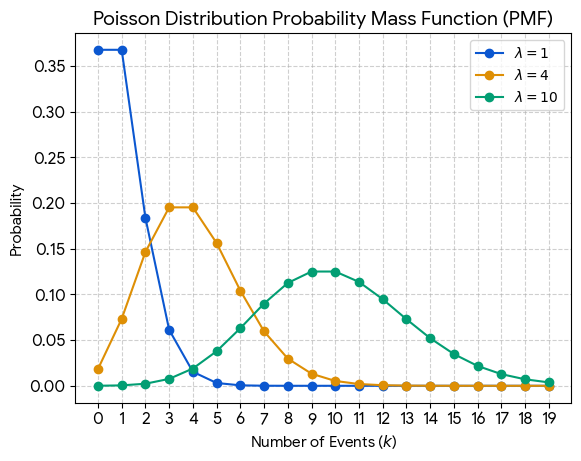
The generated graph plots the probabilities across different event counts () for three distinct values of (, , and ).
When the arrival rate is low (), the distribution exhibits heavy right-skewness. The probability peaks immediately at zero and one, restricted by the hard boundary of the y-axis because negative events are an impossibility.
As the expected rate rises to and eventually , the distribution's center of mass migrates rightward along the horizontal axis. Crucially, the curve also flattens and widens. This behavior offers direct visual proof of the distribution's core property: as the mean shifts, the variance expands at an identical rate. For larger values of , the distribution loses its initial asymmetry, organically smoothing out into a symmetrical, bell-shaped profile that closely approximates a normal distribution.